Model
The Spatiocoexistence framework provides a spatially explicit theory for understanding how ecological patterns and processes interact to shape the dynamics and coexistence of diverse forest communities. This section outlines the theoretical foundations individual-based model.
In the following we will discuss, how we calculate the:
Crowding Indices
and how we model the:
Mortality,
Recruitment,
Growth, of trees.
Crowding Indices
Crowding indices quantify the competitive pressure experienced by individual trees from their neighbors. These metrics form the foundation for understanding spatial competition in forest communities.
The framework distinguishes between two types of competitive interactions:
Conspecific Crowding (CI_CS): Competition from neighbors of the same species, representing intraspecific competition for resources. It is defined as:
with:
NN, the nearest neighbors, all neighbors within a certain distance R
\(BA_j = \pi \frac{dbh_j}{2}^2\), the basal area of the neighbor j, whereas \(dbh\) is the diatmeter at breast height
\(d_{ij}\), the distance between the individuals i, j
\(\delta_{s_is_j}\), the Kronecker delta of the species \(s_{i/j}\)
Heterospecific Crowding (CI_HS): Competition from neighbors of different species, representing interspecific competition. It is defined as:
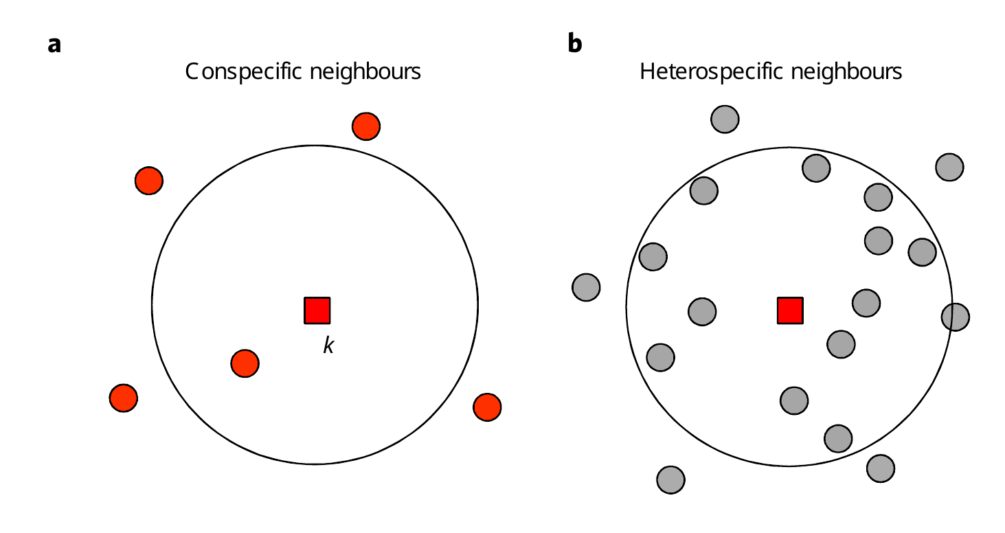
Figure 1 : This is a visualisation of the calculation of the crowding index, showing the focal tree (centre) with its conspecific neighbours (same species, red) on the left and its heterospecific neighbours (different species, grey) on the right within a radius of R.
Figure Figure 1 shows the differences in the method used to calculate the crowding indices.
Mortality
We model tree mortality as a stochastic process influenced by crowding indices. We calculate two different survival probabilities for mortality: One is for reproductive trees, which are larger than or equal to the reproductive size (\(dbh>rep\_size\)). The other is for saplings, which are smaller than reproductive trees. Then, we generate a random number and compare it with the survival probability. If the random number is larger than the survival probability, the tree dies.
With:
\(S_{rep}\), the survival parameter for reproductive trees
\(\beta_S\) and \(\beta_{HS}\) the …
Z, the random number
Survival of saplings:
Furthermore, we apply a linear decrease to the survival rate of a tree if its size exceeds a threshold (if \(dbh_i > MS\)), calculated as follows:
With
MS, the maximal size factor calculated as (ToDo)
\(dbh_{max}\), the maximal dbh we define in the model
Recruitment
The recruitment process involves determining the number of new recruits required and their distribution within the census.
First of all, the number of recruits for each species is calculated by:
With:
rep, the mean reproduction rate
A_{rep}(s), the abundance of reproductive trees of species \(s\)
Than they are distributed:
Check if: Z < BA_i / BA(s) to increase the probability of large individuals/trees becoming parent trees. This is a tree where the recruit is placed in its neighbourhood. If the parent tree has a basal area larger than the mean basal area of species s (\(\overline{BA(s)}\)), then it is clear that the tree can be used as a parent.
Draw the x, y position of a potential recruit from a 2D Gaussian distribution around the parent tree’s location.
Calculate the crowding indices of the recruit at that potential location.
Using these indices, calculate a survival probability as we did for saplings in the mortality process:
With a minimal survival probability (\(surv_{min}\)). Is the survival of that recruit (\(S_i\)) smaller than this value, we look for a new recruit.
Growth
Growth is not a stochastic process; the gain in diameter is calculated for each tree.
For each tree, we calculate its growth according to the following formula:
\(\beta_g\), …
\(\beta_{Hg}\), …
\(g\), …
\(r\), ..
Modelling of a single timestep (5 years)
The spatially explicit, individual-based model sequentially integrates all demographic processes (mortality, recruitment and growth) for each 5-year time step.
The following flowchart illustrates the complete algorithm:
        flowchart TD
    A[Get initial inventory] --> B(Calculate Crowding Indices)
    B --> C(Mortality: <br> status = -1, if dead)
    C --> |status 1 -> 0|D(Recruitment)
    D --> E(Remove deads <br> ignore i if status = -2 <br> Add recruits to inventory)
    E --> |status -1 -> -2| F(Growth <br> dbh = dbh + δdbh)
    F --> B